DesignCollaborationBetterProducts << Previous

MechatronicDesignCases

After reading this chapter the reader will:

experiment his knowledge in regard to the design and real time implementation of mechatronic systems
live the design of mechatronic systems from A to Z
be able to perform the different phases of the design of mechatronicsystems
be able to solve the control problem and establish the control law that we have to implement in real time
be able to write programs in C language using the interrupt concept for real time implementation

閱讀完本章後，讀者將：

1.實驗他在設計和實時方面的知識機電系統的實施

2.進行從A到Z的機電系統設計

3.能夠執行機電一體化設計的不同階段系統

4.能夠解決控制問題並建立控制律我們必須實時實施

5.能夠使用C語言的中斷概念編寫程序實時實施

11.1 Introduction

In the previous chapters we developed some concepts that we illustrated their appli-cations by academic examples to show the readers how these results apply. More specifically, we have seen how to design the mechatronic systems and we have presented the different steps that we must follow to success the design of the desired mechatronic system. We have presented the approaches that we must use in the design of:

the mechanical part
the electronic circuit
the program in C for the real-time implementation

在前面的章節中，我們開發了一些概念，說明了它們的應用。通過學術實例向讀者展示這些結果如何應用。更多具體來說，我們已經了解瞭如何設計機電一體化系統，並且介紹了成功完成所需目標設計所必須遵循的不同步驟機電系統。我們已經介紹了我們必須在設計：

機械部分
電子線路
C語言中用於實時執行的程序

These tools were applied for some practical systems and more details were given to help the reader to execute his own design.

這些工具已用於一些實際系統，並提供了更多詳細信息幫助讀者執行自己的設計。

For the control algorithms most of the examples we presented were academic with perfect models. Unfortunately, for a practical system the model we will have is just a realization that may describe the system in some particular conditions, and for some reasons this model will not work perfectly as expected during the real-time implementation of the algorithms. This can be caused by different neglected dynamics that may change the behavior for some frequencies.

對於控制算法，我們提供的大多數示例都是具有理想模型的學術模型。不幸的是，對於一個實際的系統，我們將擁有的模型只是一個可以在某些特定條件下描述該系統的實現，並且由於某些原因，該模型無法在算法的實時實現過程中按預期方式完美運行。這可能是由不同的被忽略的動力學引起的，這些動力學可能會改變某些頻率的行為。

The aim of this chapter is to show the reader how we can implement in real-time the theoretical results we developed earlier in the previous chapters for practical systems. We will proceed gradually and show all the steps to make it easy for the readers. The case studies we consider in this chapter are those that are discussed and designed in the previous chapters.

本章的目的是向讀者展示我們如何實時實現前面幾章中針對實際系統開發的理論結果。我們將逐步進行並顯示所有步驟，以使讀者輕鬆閱讀。我們在本章中考慮的案例研究是在前幾章中討論和設計的案例研究。

11.2 Velocity Control of the dc Motor Kit

As a first example, let us consider the speed control of the dc motor driving a me-chanical part. The choice of this example is very important since most of the systems will use such dc motor. The dc motor we will consider is manufactured by Maxon company. This motor is very important since it comes with a gearbox (ratio 6:1) and an encoder that gives one hundred pulses per revolution, which gives 600 pulses per revolution that we exploit by using quadrature method to bring it to two thousand four hundred pulses per revolution. The system we are using in this example for the real-time implementation of control algorithms we presented earlier if more flexible and offer more advantages.

作為第一個示例，讓我們考慮驅動機械零件的直流電動機的速度控制。該示例的選擇非常重要，因為大多數係統將使用此類直流電動機。我們將考慮的直流電動機由Maxon公司製造。該電動機非常重要，因為它帶有齒輪箱（比率6：1）和編碼器，該編碼器每轉給出一百個脈衝，我們每轉產生600個脈衝，我們通過使用正交方法將其變為24400個脈衝。每轉。本示例中使用的系統用於實時實現控制算法，如果更靈活並且具有更多優勢，我們將在前面介紹。

The data sheet of this motor gives all the important parameters and therefore the transfer function of this actuator can be obtained easily. The load we are considering in this example is a small disk with graduation that we would like to control in speed and later on in position. This setup is illustrated in Figs. 11.1-(11.2). The disk we are considering has a diameter equal to 0.06 m and a mass equal to 0.050 Kg. With these data and the one of the data sheet of the dc motor, we can get the transfer function between the velocity of the disk and the input voltage.

該電動機的數據表提供了所有重要參數，因此可以輕鬆獲得該執行器的傳遞函數。在此示例中，我們正在考慮的負載是一個帶有刻度的小磁盤，我們希望在速度上控制它，然後在位置上進行控制。這種設置在圖1和2中示出。 11.1-（11.2）。我們正在考慮的圓盤的直徑等於0.06 m，質量等於0.050 Kg。利用這些數據和直流電動機的數據表之一，我們可以獲得磁盤速度和輸入電壓之間的傳遞函數。

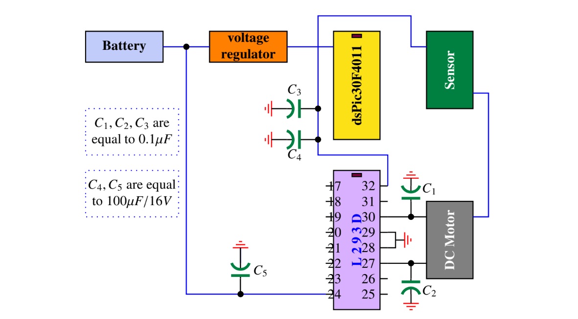
Fig. 11.1 Electronic circuit of dc motor kit

or proceed with an identification. Using the first approach the results of Chapter 2 in [1], we get:

或繼續進行識別。使用第一種方法，[1]中第2章的結果是：

For the identification of our system, we can do it in real-time using the real- time implementation setup and appropriate C program. Since the microcontroller owns limited memory, the identification can be done into two steps. Firstly, in a first experiment the gain, K, is determined, then using this gain we compute the steady state value that can be used to compute the constant time τ.

為了識別我們的系統，我們可以使用實時實施設置和適當的C程序實時進行識別。由於微控制器擁有有限的存儲器，因此識別可以分為兩個步驟。首先，在第一個實驗中，確定增益K，然後使用該增益來計算可用於計算恆定時間τ的穩態值。

To design the controller we should first of all specify the performances we would like that our system has. As a first performance, we require that our system is stable. It is also needed that the system speed will have a good behavior at the transient regime with a zero error at the steady state regime for a step reference. For the transient we would like that our load has a settling time with 5% less or equal to 3τ/5 and an overshoot less or equal to 5%.

為了設計控制器，我們首先應該指定我們希望系統具有的性能。作為首要性能，我們要求系統穩定。還需要係統速度在瞬態狀態下具有良好的性能，並且在穩態狀態下的零誤差作為階躍參考。對於瞬態，我們希望負載的穩定時間小於或等於3τ/ 5 5％，而過衝則小於或等於5％。

To accomplish the design of the appropriate controller we can either make the design in continuous-time and then obtain the algorithm we should program in the software part, or proceed with all the design in the discrete-time directly. In the rest of this example, we will opt for the second approach.

為了完成適當控制器的設計，我們既可以連續進行設計，然後獲得應在軟件部分進行編程的算法，也可以直接在離散時間內進行所有設計。在本示例的其餘部分中，我們將選擇第二種方法。

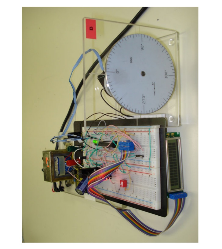
Fig. 11.2 Real-time implementation setup

From the expression of the system transfer function, and the desired perfor-mances it results that we need at least a proportional and integrator (PI) controller.

從系統傳遞函數的表達式以及所需的性能來看，我們至少需要一個比例積分器（PI）控制器。

The transfer function of this controller is given by:

該控制器的傳遞函數由下式給出：

where KP and KI are gains to be determined to force the load to have the performances we imposed.

其中KP和KI是要確定的結果，以迫使負載具有我們施加的性能。

Using a zero-order-holder and the Z -transform table we get:

使用零序持有者和Z -transform表，我們得到：

For the controller, using the trapezoidal discretisation we get:

對於控制器，使用梯形離散化，我們得到：

Dividing the numerator and the denominator by z and going back to time, we get:

將分子和分母除以z並回到時間，我們得到：

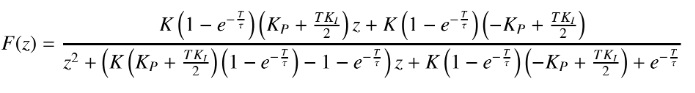
Combining the transfer function of the actuator and its load and the one of the controller we get the following closed-loop transfer function:

結合執行器及其負載和控制器之一的傳遞函數，我們得到以下閉環傳遞函數：

Using now the desired performances, it is easy to conclude that the dominant poles are

現在使用期望的性能，很容易得出結論，主導極點是

where ζ and ωn represent respectively the damping ratio and the natural frequency of the closed-loop of our system control.

其中ζ和ωn分別代表我們系統控制閉環的阻尼比和固有頻率。

From control theory (see Boukas [1]) it is well known that the overshoot d% and the settling time ts at 5% are given by:

根據控制理論（請參見Boukas [1]），眾所周知，過衝d％和5％的建立時間ts由下式給出：

Using our performances and these expressions we conclude that:

使用我們的表演和這些表達，我們得出以下結論：

which give the following dominant poles:

它具有以下主要優勢：

Using the transformation z = eT s with T = τ/10 = 0.0064, we obtain the following dominant poles in the Z -domain:

使用Z = eT s且T =τ/ 10 = 0.0064的變換，我們在Z域中獲得以下主導極點：

Using now the poles placement technique we get:

現在使用極點放置技術，我們得到：

which implies:

這意味著：

Using the values of K, T and τ, we get the following expression for the gains KP and KI:

使用K，T和τ的值，我們得到增益KP和KI的以下表達式：

Remark 11.2.1 Cautions have to be made in this case since we don’t care about the positions of the zero of the transfer function and therefore we may have some surprises when implementing this controller. It is clear that the performances we will get (settling time and the overshoot) will depend on the positions of the zero. For more details on this matter we refer the reader to Boukas [1].

備註11.2.1在這種情況下，必須謹慎，因為我們不在乎傳遞函數零的位置，因此在實現此控制器時可能會有些意外。顯然，我們將獲得的性能（穩定時間和過衝）將取決於零的位置。有關此問題的更多詳細信息，請向讀者介紹Boukas [1]。

To implement now this PI control algorithm and assure the desired performances we will use a microcontroller from Microship1. This choice is due to our experience with this type of microcontroller. The reader can keep in mind that any other micro-controller from other manufacturer with some small changes will do the job. In this example we will use the microcontroller dsPIC30F4011 from Microhip.

為了實現此PI控制算法並確保所需的性能，我們將使用Microship1的微控制器。這種選擇是由於我們在此類微控制器方面的經驗所致。讀者可以記住，其他製造商的任何其他微控制器只要稍作改動，就可以完成工作。在本示例中，我們將使用Microhip的單片機dsPIC30F4011。

The code for our implementation is made in C-language. This language is adopted for its simplicity. The implementation has the following structure:

我們實現的代碼使用C語言編寫。採用這種語言是因為其簡單性。該實現具有以下結構：

// Put here the include

#include "p30F4011.h" // proc specific header

// Define a struct

typedef struct {

// PI Gains

float K_P; // Propotional gain

float K_I; // Integral gain

// PI Constants

float Const1_pid; // KP + T KI/2

float Const2_pid; // -KP + T KI/2

float Reference; // speed reference

// System variables

float y_k; // y_m[k] -> measured output at time k

float u_k; // u[k] -> output at time k

float e_k; // e[k] -> error at time k

// System past variables

float u_prec; // u[k-1] -> output at time k-1

float e_prec; // e[k-1] -> error at time k-1

}PIStruct;

PIStruct thePI;

thePI.Const1= thePI.K_P+T*thePI.K_I/2;

thePI.Const2=-thePI.K_P+T*thePI.K_I/2;

thePI.Reference=600;

// Functions

float ReadSpeed(void);

float ComputeControl(void);

float SendControl(void);

// Interrupt program here using Timer 1 (overflow of counter Timer 1)

void __ISR _T1Interrupt(void) // interrupt routine code

{

// Interrupt Service Routine code goes here

float Position_error;

// Read speed

thePI.y_m=ReadSpeed();

thePI.e_k= thePI.Reference-thePI.y_m;

// Compute the control

ComputeContrl();

// Send control

SendControl();

IFS0bits.T1IF=0; // Disable the interrupt

}

int main ( void ) // start of main application code

{

// Application code goes here

int i;

// Initialize the variables Reference and ThePID.y_m (it can be read

from inputs) Reference = 0x8000; // Hexadecimal number

(0b... Binary number) ThePID = 0x8000;

// Initialize the registers

TRISC=0x9fff; // RC13 and RC14 (pins 15 and 16) are configured as outputs

IEC0bits.T1IE=1; // Enable the interrupt on Timer 1

// Indefinite loop

while (1)

{

}

return 0

}

% ReadSpeed function

int ReadSpeed (void)

{

}

% ComputeControl function

int ComputeControl (void)

{

thePI.u_k=thePI.u_prec+thePI.Const1*thePI.e_k+thePI.Const2*thePI.e_prec;

}

% SendControl function

int Send Control (void)

{

sendControl()

// Update past data

thePI.u_prec=thePI.u_k;

ThePI.e_prec=thePI.e_k;

}

As it can be seen from this structure, first of all we notice that the system will enter the loop and at each interrupt the call for the functions:

ReadSpeed;
ComputeControl;
SendControl;

is made and the appropriate action is taken.

從該結構可以看出，首先我們注意到系統將進入循環，並在每次中斷時調用函數：

ReadSpeed；
ComputeControl；
SendControl；

並採取適當的措施。

The ReadSpeed function returns the load speed at each sampling time that will be used by the ComputeControl function. The SendControl function sends the appropriate voltage to the actuator via the L293D chip.

ReadSpeed函數在每個採樣時間返回加載速度，該速度將由ComputeControl函數使用。 SendControl功能通過L293D芯片將適當的電壓發送到執行器。

Using the compiler HighTec C to get the hex code and the PicKit-2 to upload the file in the memory of the microcontroller. For more detail on how to get the hex code we invite the reader to the manual of the compiler HighTec C or the compiler C30 of Microchip.

使用編譯器HighTec C獲取十六進制代碼，並使用PicKit-2將文件上傳到微控制器的內存中。有關如何獲取十六進制代碼的更多詳細信息，我們邀請讀者閱讀編譯器HighTec C或Microchip的編譯器C30的手冊。

The state approach in this case is trivial and we will not develop it.

在這種情況下，國家方法是微不足道的，我們將不發展它。

11.3 Position Control of the dc Motor Kit

Let us focus on the load position control. Following similar steps as for the load ve-locity control developed in the previous section, we need firstly to choose the desired performances we would like our system will have. The following performances are imposed:

system stable in the closed-loop;
settling time ts at 2% equal to the best one we can have
overshoot equal to 5%
steady-state equal to zero for a step function as input

讓我們專注於負載位置控制。遵循與上一節中開發的負載速度控制類似的步驟，我們首先需要選擇我們希望系統具有的理想性能。進行以下表演：

系統穩定在閉環狀態；
穩定時間ts為2％，等於我們可以擁有的最佳時間
超調等於5％
步進功能作為輸入的穩態等於零

Using the performances and the transfer function, it is easy to conclude that a proportional controller KP is enough to satisfy these performances.

使用性能和傳遞函數，很容易得出結論，比例控制器KP足以滿足這些性能。

In this example, we will use the continuous-time approach for the design of the controller. Based on the past chapter, the model of our system is given by:

在此示例中，我們將使用連續時間方法進行控制器的設計。在上一章的基礎上，我們的系統模型如下：

where K and τ take the same values as for the speed control.Let the transfer controller be give by:

其中K和τ的取值與速度控制的取值相同。

Using these expression, the closed-loop transfer function is given by:

使用這些表達式，閉環傳遞函數由下式給出：

Since the system is of type 1, it results that the error to a step function as input is equal to zero with a proportional controller.Based on the specifications, the following complex poles:

由於系統類型為1，因此使用比例控制器時，輸入階躍函數的誤差等於零。根據規格，以下複雜極點：

will do the job and the corresponding characteristic equation is given by:

將完成這項工作，相應的特徵方程式如下：

Equating this with the one of the closed-loop system we get:

與閉環系統之一等效，我們得到：

To determine the best settling time ts at 2 %, notice that we have:

為了確定最佳穩定時間ts為2％，請注意，我們有：

Using now the fact:

現在使用事實：

we obtain:

我們獲得：

Therefore the best settling time at %2 we can have with this controller is 8 times the constant time of the system. Any value less than will be attainable. In fact, this is trivial if we look to the root locus of the closed-loop system when varying KP. This is given by Fig. 11.3. To fix the gain of the controller the desired poles s1,2 = −7.5±j, we use the figure and choosing a ζ = 0.707. This gives KP = 0.1471.

因此，使用此控制器可以在％2處獲得的最佳建立時間是系統恆定時間的8倍。小於可獲得的任何值。實際上，如果我們在改變KP時關注閉環系統的根源，這是微不足道的。這由圖11.3給出。為了將控制器的增益固定為所需的極點s1,2 = -7.5±j，我們使用該圖並選擇ζ= 0.707。得出KP = 0.1471。

Fig. 11.3 Root locus of the dc motor with a proportional controller

Using this controller, the time response for a step function of amplitude equal to 30 degrees is represented by the Fig. 11.4 from which we conclude that the designed controller satisfies all the desired performances with a settling time at %2 equal to 0.5115 s. But if we implement this controller, the reality will be different from simulation since the backlash of the gearbox is not included in the used model and therefore in real-time the result will be different and the error will never be zero. To overcome this problem we can use a proportional and derivative controller that may give better settling time at %2. Let the transfer function of this controller be given by:

使用該控制器，幅度等於30度的階躍函數的時間響應由圖11.4表示，從中我們可以得出結論，所設計的控制器以％2的穩定時間等於0.5115 s滿足了所有期望的性能。但是，如果我們實現此控制器，則實際情況將與仿真有所不同，因為變速箱的齒隙並未包含在所使用的模型中，因此實時結果將有所不同，誤差永遠不會為零。為了克服這個問題，我們可以使用比例和微分控制器，它可以在％2處提供更好的建立時間。讓該控制器的傳遞函數由下式給出：

where KP and KD are the gain to be determined.

其中KP和KD是要確定的增益。

Remark 11.3.1 It is important to notice that the use of a proportional and deriva-tive controller will introduce a zero in the closed-loop transfer that may improve the settling time if it is well placed. Depending on its position, the overshoot and the settling time will be affected. For more details on this matter we refer the reader to [1].

備註11.3.1必須注意，使用比例和微分控制器會在閉環傳遞中引入零，這可能會改善放置時間是否合適。根據其位置，過沖和建立時間將受到影響。有關此問題的更多詳細信息，請參考[1]

Fig. 11.4 Time response for a step function with 30 degrees as amplitude

With this controller the closed-loop transfer function is given by:

使用該控制器，閉環傳遞函數由下式給出：

As before two complex poles are used for the design of the controller. If we equate the two characteristic equations we get:

和以前一樣，控制器的設計使用了兩個複雜的極點。如果將兩個特徵方程式相等，則得到：

In this case we have two unknown variables KP and KD and two algebraic equations which determines uniquely the gains. Their expressions are given by:

在這種情況下，我們有兩個未知變量KP和KD以及兩個唯一確定增益的代數方程。它們的表達式如下：

Using now the desired performances, we conclude similarly as before that the steady error to an input equal to step function of amplitude equal to 30 degrees for instance is equal to zero and the damping ratio ζ corresponding to an overshoot equal to %5 is equal to 0.707. The settling time, ts at % 2, that we may fix as a proportion of the time constant of the system, gives:

現在，使用期望的性能，我們得出與之前類似的結論，即等於等於30度的幅度階躍函數的輸入的穩態誤差等於零，並且與過衝等於％5的阻尼比ζ等於0.707。我們可以將其固定為系統時間常數的一部分的穩定時間ts在％2處給出：

Now if we fix the settling time at 3τ, we get:

現在，如果將穩定時間固定為3τ，我們將得到：

Using these values we get the following ones for the controller gains:

使用這些值，我們可以得到以下控制器增益值：

which gives the following complex poles:

它給出了以下複雜的兩極：

and the zero at:

零為：

Using this controller the time response for an input with an amplitude equal to 30 degrees is represented in Fig. 11.5. As it can be seen from this figure that the overshoot and the settling time are less those obtained using the proportional controller.

使用該控制器，幅度等於30度的輸入的時間響應如圖11.5所示。從該圖可以看出，過沖和建立時間少於使用比例控制器獲得的過沖和建立時間。

To implement either the proportional or the proportional and derivative con-trollers we need to get the recurrent equation for the control law. For this purpose, we need to discretize the transfer function of the controller using the different meth-ods presented earlier. Let us use the trapezoidal method which consists to replace s by 2(z−1)/T(z+1) . This gives:

為了實現比例控制器或比例控制器和微分控制器，我們需要獲得控制律的遞推方程。為此，我們需要使用前面介紹的不同方法來離散化控制器的傳遞函數。讓我們使用梯形方法，該方法包括將s替換為2（z-1）/ T（z + 1）。這給出：

If we denote by u(k) and e(k) by the control and the error between the reference and the output at instant kT, we get the following expressions:

for the proportional

如果我們通過控制分別表示u（k）和e（k）以及在瞬時kT處參考和輸出之間的誤差，我們將得到以下表達式：

1.比例

u(k) = KPe(k)

for the proportional and derivative controller

2.用於比例和微分控制器

u(k) = −u(k − 1) + (KP + 2KD/T) e(k) + (KP − 2KD/T) e(k − 1)

The implementation is this controller uses the same function with some minors changes. The listing the corresponding functions is:

實現是該控制器使用相同的功能，但有一些小的更改。列出相應的功能是：

%%%%%%%%%%%%%%%%%%%%%%%%%%%%%%%%%%%

% Main program %

%%%%%%%%%%%%%%%%%%%%%%%%%%%%%%%%%%%

main

% Data

% Variables

% While loop

while (1)

ReadSpeed;

ComputeControl;

SendControl;

end;

% ReadSpeed function

% ComputeControl function

% SendControl function

Let us now use the state space representation of this example and design a state feedback controller that will guarantee the desired performances. For this case we will firstly assume the complete access to the states and secondly we relax this as-sumption by assuming that we have access only to the position. As we did previously we can proceed either in the continuous-time or in discrete-time. Previously we establish the state space description of this system and it is given by:

現在讓我們使用此示例的狀態空間表示，並設計一個狀態反饋控制器，以保證所需的性能。對於這種情況，我們將首先假定完全訪問狀態，其次通過假定我們只能訪問該職位來放寬此假設。像我們之前所做的那樣，我們可以連續進行，也可以不連續進行。先前我們建立了該系統的狀態空間描述，其描述為：

where x(t) ∈ R2 (x1(t) = θ(t) and x2(t) = θ ̇(t)), and u(t) ∈ R (the applied voltage). From the desired performances with a settling time at %2 equal to 3τ, we get the same dominant poles as before, and therefore the same characteristic equation, Δd(s) = s*s + 2ζwn s + w2/n = 0 (with ζ = 0.707 and wn = 4/3ζτ ). Using the controller expression the closed-loop characteristic equations given by:

其中x（t）∈R2（x1（t）=θ（t）和x2（t）=θ̇（t）），u（t）∈R（施加電壓）。從穩定時間為％2等於3τ的期望性能中，我們得到與以前相同的主導極點，因此具有相同的特性方程Δd（s）= s * s +2ζwns + w2 / n = 0（ ζ= 0.707，wn = 4 /3ζτ）。使用控制器表達式，閉環特性方程由下式給出：

det (sI − A + BK) = 0

By equalizing these two equations we get the following gains:

通過均衡這兩個方程式，我們可以得到以下收益：

K1 = 1.1146

K2 = 0.0326

Using this controller the time response for an input with an amplitude equal to 30 degrees is represented in Fig. 11.6. As it can be seen from this figure that the overshoot and the settling time are those we would like to have. It is important to notice the existence of the error at the steady state regime. This error can be eliminated if we add an integral action in the loop. For more detail on this we refer the reader to [1].

使用該控制器，幅度等於30度的輸入的時間響應如圖11.6所示。從該圖可以看出，超調和建立時間就是我們想要的。重要的是要注意穩態狀態下錯誤的存在。如果在循環中添加一個積分動作，則可以消除此錯誤。有關此的更多詳細信息，請向讀者介紹[1]。

For the second case since we don’t have access to the load speed we can either compute it from the position or use an observer to estimate the system state. As it was said earlier, the poles that we use for the design of the observer should be faster than those used in the controller design.

對於第二種情況，由於我們無法獲得負載速度，因此我們可以從位置計算負載速度，也可以使用觀察者來估算系統狀態。如前所述，我們用於觀察者設計的極點應該比控制器設計中使用的極點更快。

we get the following gains for the observer:

我們為觀察者帶來以下收益：

L1 = 151.2

L2 = 5029.4

The gains of the controller remain the same as for the complete access case to the state vector.

控制器的增益與對狀態向量的完全訪問情況相同。

In the following Matlab we provide the design of the controller and the observer at the same time and give simulation that shows the behavior of the states of the system and observer with respect to time.

在下面的Matlab中，我們同時提供控制器和觀察者的設計，並進行仿真，以顯示系統和觀察者的狀態相對於時間的行為。

clear all

%data

tau=0.064

k=48.9

A = [0 1;0 -1/tau];

B = [0 ; k/tau];

C = [1 0];

D = 0;

% controller design

K = acker(A,B,[-3+3*j -3-3*j]);

L = acker(A’,C’,[-12+3*j -12-3*j])’;

% Simualation data

Ts = 0.01;

x0 = [1 ; 1];

z0 = [1.1 ; 0.9];

Tf = 2; %final time

%augmented system

Ah = [A -B*K;

L*C A-B*K-L*C];

Bh = zeros(size(Ah,1),1);

Ch = [C D*K];

Dh = zeros(size(Ch,1),1);

xh0 = [x0 ; z0];

t=0:Ts:Tf;

u = zeros(size(t));

m = ss(Ah,Bh,Ch,Dh);

%simulation

[y,t,x] = lsim(m,u,t,xh0);

%plotting

figure;

plot(t,y);

title(’Output’);

xlabel(’Time in sec’)

ylabel(’Output’)

grid

figure;

plot(t,x(:,1:size(A,1)));

title(’States of the system’);

xlabel(’Time in sec’)

ylabel(’System states’)

grid

figure;

plot(t,x(:,size(A,1)+1:end));

title(’states of the observer’);

xlabel(’Time in sec’)

ylabel(’Observer states’)

grid

Figs. (11.7)-(11.9) gives an illustration of the output, the system’s states and the observer’s states.

無花果（11.7）-（11.9）給出了輸出，系統狀態和觀察者狀態的說明。

Remark 11.3.2 In general, there is no magic rule for the choice the matrices for the cost function. But in general the fact that we use a high value for the control for instance will force the control to take small values and may prevent saturation. Using these matrices and the Matlab function, lqr, we get:

備註11.3.2通常，對於成本函數的矩陣選擇沒有魔術規則。但是通常，例如，我們對控件使用較高的值將迫使控件採用較小的值，並可能防止飽和。使用這些矩陣和Matlab函數lqr，我們得到：

K =0.3162 0.6875

We can also design a state feedback controller using the results on robust control part. Since the system has no uncertainties and there is no external disturbance, we can design a state feedback controller for the nominal dynamics. Using the system data and Maltlab, we get:

我們還可以使用魯棒控制部分的結果設計狀態反饋控制器。由於系統沒有不確定性，也沒有外部干擾，所以我們可以為名義動態設計一個狀態反饋控制器。使用系統數據和Maltlab，我們得到：

X = 1.1358 −0.3758

−0.3758 1.1465

Y = −0.0092 0.0228

The corresponding controller gain is given:

給出了相應的控制器增益：

K =−0.0017 0.0193

Remark 11.3.3 Since we have the continuous-time model for the dc motor kit, we have use it to design the controller gain. In this case we have solved the following LMI:

備註11.3.3由於我們有直流電動機套件的連續時間模型，因此我們用它來設計控制器增益。在這種情況下，我們解決了以下LMI：

AX + XA + BY + YB < 0

The gain K is given by: K = YX−1.

增益K由下式得出：K = YX-1。

For more detail on the continuous time case we refer the reader to Boukas [2] and the references therein.

有關連續時間情況的更多詳細信息，請向讀者介紹Boukas [2]及其中的參考文獻。

DesignCollaborationBetterProducts << Previous